DEVISE API R Example

For this example, we provide some basic example workflows to accessing, querying and even downloading climate data available within the DEVISE cyberinfrastructure. We use DEVISE API’s to query for existing climate summary data that are stored within the ARCC S3 Pathfinder storage server as Cloud Optimized GeoTiffs (COGs).

Before reading this example users should look over the DEVISE API, User Interface, and dataset documentation to understand what each element provides.

Using R with DEVISE Data

For the below examples we will want to use Program R and have the following Packages installed. If you do not have any of the following packages installed, the following code should get you started.

Also this custom datatable function render_datatable is nice for viewing json lists.

install.packages(c("sf", "terra", "lubridate", "httr", "jsonlite", "tidyverse", "tidyjson", "plotly", "kableExtra", "DT", "mapview"))

# A helpful custom visualize function
render_datatable <- function(data_list, sort_col_index = 0) {
  datatable(
    data_list, 
    options = list(
      pageLength = 3,
      autoWidth = FALSE,
      scrollX = FALSE,
      order = list(list(sort_col_index, 'asc'))
    ), 
    rownames = FALSE,
    class = 'cell-border stripe hover'
  )
}

---

Once you have the correct packages installed, let’s load them into our session so we can do some work.

Now that our environment is prepared, let’s first check out the available datasets and the associated timeseries incrementations:

response <- GET("https://devise.uwyo.edu/Timescale", add_headers(Accept = "application/json"))

data_list <- fromJSON(content(response, as = "text", encoding = "UTF-8"), flatten = TRUE)

render_datatable(data_list, sort_col_index = 1)

---

In order to better understand each dataset lets review their unique variables.

response <- GET("https://devise.uwyo.edu/Variables", add_headers(Accept = "application/json"))
data_list <- fromJSON(content(response, as = "text", encoding = "UTF-8"), flatten = TRUE) %>%
  select(dataset, variable, alias, units, description, scaleFactor)

render_datatable(data_list)

There are a lot of different variables and it is important to note that there is a Scale Factor we need to pay attention to (we will need to adjust the resulting values accordingly).

---

Another property to keep in mind is the resolution for each dataset. Lets take a look at PRISM’s tmean cell size resolution. What sort of cell size is ideal for a project.

response <- GET("https://devise.uwyo.edu/GetS3Urls", add_headers(Accept = "application/json"))
data_list_2 <- fromJSON(content(response, as = "text", encoding = "UTF-8"), flatten = TRUE) %>%
  select(filename, variable, resolution)

render_datatable(data_list)

---

OK, we have a pretty good idea of the available datasets, let’s learn how to interact with them given that there are several methods!

Since the climate data are COGs, we can query them spatially from the cloud and not have to worry about downloading files. To do this let’s first add some polygons to our environment….let’s go with the Counties of Wyoming from the ESRI Feature Service. Notice that we add an ID column that matches row.names() of the layer. We will use this later on in our processing.

url<- parse_url("https://services.arcgis.com/P3ePLMYs2RVChkJx/ArcGIS/rest/services/USA_Boundaries_2022/FeatureServer/2/query")

url$query <- list(where = "STATE_FIPS='56'",
                  outFields = "*",
                  returnGeometry = "true",
                  f = "geojson")
request <- build_url(url)

county <- st_read(request) %>% 
  mutate(ID = as.integer(rownames(.)))

Reading layer `OGRGeoJSON' from data source 
  `https://services.arcgis.com/P3ePLMYs2RVChkJx/ArcGIS/rest/services/USA_Boundaries_2022/FeatureServer/2/query?where=STATE_FIPS%3D%2756%27&outFields=%2A&returnGeometry=true&f=geojson' 
  using driver `GeoJSON'
Simple feature collection with 23 features and 14 fields
Geometry type: POLYGON
Dimension:     XY
Bounding box:  xmin: -111.0546 ymin: 40.99478 xmax: -104.0523 ymax: 45.00582
Geodetic CRS:  WGS 84

ggplot(county) + 
  geom_sf()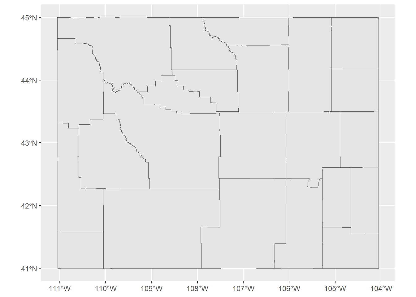

Let’s look at the PRISM dataset variable Annual Mean Temperature for Albany County for the entire timeseries. First we need to obtain the URLs for the specified variable and timescale (notice the query parameters within the URL).

cogs<- GET("https://devise.uwyo.edu/GetS3Urls?Variable=tmean&Dataset=PRISM&Timescale=annual") %>% 
  content() %>% 
  spread_all() %>% 
  data.frame()

---

Now that we know which data we are querying (annual estimates of mean temperature from the PRISM dataset) and where the data is located (urlCOG), we are all set to conduct some raster analyses using cloud resources! First we stack the rasters, then we extract the mean of all cells within our polygon boundary (filtering for Albany County) for each layer (each year). Be sure to use the URL with vsicurl prefix AND to adjust the raster values by the scale factor!

# Access the data virtually as opposed to downloading with the the prefix /vsicurl/
rs<- rast(paste0("/vsicurl/", cogs$url), vsi = TRUE)

scale_factor <- cogs$scale

e<- terra::extract(rs, county %>% 
                     filter(FIPS %in% c("56001")), fun = mean) %>% 
  pivot_longer(2:ncol(.), names_to = "raster", values_to = "value") %>% 
  mutate(sampDate = as.Date(paste0(str_extract(raster, "\\d{4}"), "-01-01"))) %>%
  left_join(county %>% 
              select(ID, NAME:FIPS), by = "ID") %>% 
  mutate(value = value * scale_factor)

Now lets plot the results!

ggplotly(
  e %>% 
    ggplot(aes(x = sampDate, y = value, group = NAME, color = NAME)) +
    geom_line() +
    ylab(paste(cogs$alias[1], cogs$units[1])) +
    scale_x_date(
      date_breaks = "10 years", 
      date_labels = "%Y"          
    ) +
    theme_classic()
)

---

Lets add all the counties in Wyoming not just Albany County!

eAll<- terra::extract(rs, county, fun = mean) %>% 
  pivot_longer(2:ncol(.), names_to = "raster", values_to = "value") %>% 
  mutate(sampDate = as.Date(paste0(str_extract(raster, "\\d{4}"), "-01-01")))  %>%
  left_join(county %>% 
              select(ID, NAME:FIPS), by = "ID") %>% 
  mutate(value = value * scale_factor)

ggplotly(
  eAll %>% 
    ggplot(aes(x = sampDate, y = value, color = NAME)) +
    geom_line() +
    ylab(paste(cogs$alias[1], cogs$units[1])) +
    scale_x_date(
      date_breaks = "10 years",
      date_labels = "%Y"
    ) +
    theme_classic()
)

---

There are enough counties in Wyoming that last one is hard to distinguish. Here is a heatgraph to allow us to easily tell which Wyoming counties are hot or cold relative to each other.

eAll<- terra::extract(rs, county, fun = mean) %>% 
  pivot_longer(2:ncol(.), names_to = "raster", values_to = "value") %>% 
  mutate(sampDate = as.Date(paste0(str_extract(raster, "\\d{4}"), "-01-01")))  %>%
  left_join(county %>% 
              select(ID, NAME:FIPS), by = "ID") %>% 
  mutate(value = value * scale_factor)

ggplotly(
  eAll %>%
    ggplot(aes(x = sampDate, y = NAME, fill = value)) +
    geom_tile() +
    scale_fill_viridis_c(name = paste(cogs$alias[1], cogs$units[1]), option = "C") +
    scale_x_date(
      date_breaks = "10 years",
      date_labels = "%Y"
    ) +
    labs(x = "Year", y = "County") +
    theme_minimal())

---

library(viridisLite)
wy_counties <- county %>% filter(substr(FIPS, 1, 2) == "56")

cogs <- GET("https://devise.uwyo.edu/GetS3Urls?Variable=tmean&Dataset=PRISM&Timescale=annual") %>% 
  content(as = "parsed") %>% 
  bind_rows() %>% 
  mutate(urlCOG = paste0("/vsicurl/", url))

rs <- rast(cogs$urlCOG, vsi = TRUE)

rs_wy <- crop(rs, vect(wy_counties))

rs_wy_scaled <- rs_wy * cogs$scale

mapview(rs_wy_scaled,
        layer.name = paste0("PRISM Tmean ", cogs$startyear[1], " (°C)"),
        col.regions = viridis(100),
        legend = TRUE) +
  mapview(wy_counties, alpha = 0, color = "black", lwd = 1)

---

What if we wanted a similar heat map for the entire western US.

mapview::mapview(rs * cogs$scale, layer.name = "2024 Mean Temp (C)")